

I wanted to do image recognition and had just started learning AI-related topics. It took me several days to understand some basic concepts, such as the differences between machine learning and deep learning. How do you do image recognition? Mainly through convolutional neural networks (CNNs). What is convolution? What is a network? These basics can be cleared up in about a day, provided you have a good tutorial. I recommend AI By Doning
Then follow the examples and implement a convolutional neural network once. You need to pay attention to the code details; otherwise you may fall into the trap of feeling like you understand everything but being unable to write anything.
1. Machine Learning, Deep Learning, and Neural Networks
Machine learning is one way to achieve artificial intelligence. Deep learning falls under machine learning, and artificial neural networks fall under deep learning. Artificial neural networks include convolutional neural networks, recurrent neural networks, and more.
Convolutional neural networks are commonly used for image classification and recognition. Recurrent neural networks are commonly used for NLP (natural language processing).
Concept reference and explanation
2. Introduction to Convolutional Neural Networks
Convolutional neural networks are mainly used for image recognition. Convolution is used to extract image features. There is something called a convolution kernel; by setting different kernel parameters, you can scan the image row by row or across multiple rows to extract features, and then use a neural network for classification.
A detailed introduction to convolution is not the focus of this article. See here for reference.
3. Structure of a Convolutional Neural Network
A typical convolutional neural network includes:
- Convolutional layer — performs convolution on the image via convolution kernels;
- Pooling layer — downsamples the image, including average pooling and max pooling;
- Fully connected layer — performs classification and prediction.
4. Classic Convolutional Neural Networks
Examples include:
LeNet — LeNet-5 is an early classic convolutional neural network. Yann LeCun created it in 1998 to recognize handwritten digits on U.S. checks.
AlexNet — It stood out at the 2012 ImageNet competition, improving image recognition accuracy by about 10% over second place. One of its authors is OpenAI / ChatGPT scientist Ilya Sutskever (now departed).
If you are interested, look up the relationships among the inventors of these networks—they may be mentors, friends, or colleagues. Many now hold senior roles at major companies, working on cutting-edge AI.
There are many others, such as VGG, GoogleNet, and ResNet. These networks are the result of arranging and optimizing different convolutional and pooling layers in different combinations. The underlying principles remain the same.
5. Building a Convolutional Neural Network
This is the focus of the article. Using LeNet-5 as an example, its structure is relatively simple. Once you understand it, you have an intuitive grasp of convolutional neural networks and are basically getting started. The prerequisite is to fully understand the code and the details, then expand from there to unfamiliar topics and gradually become comfortable with and apply neural networks.
See here for the detailed workflow. This article mainly explains key pieces of code.
5.1. LeNet Network Structure
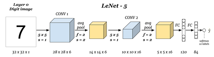
5.2. Data Loading and Preprocessing
This mainly uses Python to read raw data, get familiar with the code, and deepen your Python skills.
import gzip
import numpy as np


def read_mnist(images_path, labels_path):
    with gzip.open("MNIST_data/" + labels_path, "rb") as labelsFile:
        y = np.frombuffer(labelsFile.read(), dtype=np.uint8, offset=8)

    with gzip.open("MNIST_data/" + images_path, "rb") as imagesFile:
        X = (
            np.frombuffer(imagesFile.read(), dtype=np.uint8, offset=16)
            .reshape(len(y), 784)
            .reshape(len(y), 28, 28, 1)
        )

    return X, y


train = {}
test = {}

train["X"], train["y"] = read_mnist(
    "train-images-idx3-ubyte.gz", "train-labels-idx1-ubyte.gz"
)
test["X"], test["y"] = read_mnist(
    "t10k-images-idx3-ubyte.gz", "t10k-labels-idx1-ubyte.gz"
)

train["X"].shape, train["y"].shape, test["X"].shape, test["y"].shape
The output is a 4-dimensional tensor. A tensor can be thought of as a multi-dimensional array. Reference
((60000, 28, 28, 1), (60000,), (10000, 28, 28, 1), (10000,))
Key code explanation:
# gzip.open is a Python function for handling gzip-compressed files:

# Opens a gzip-compressed file and supports read/write operations.
# When reading, it automatically decompresses the content; when writing, it automatically compresses with gzip.
# Parameters are similar to open, with mode specifying the operation mode (e.g., "rb" for binary read).
# Commonly used for compressed log files or data archives.

# # --------------------------------------------------------------------

# The with statement in Python is used for context management of resources, ensuring they are acquired and released correctly:

# Simplifies resource management: automatically handles acquisition and release.
# Improves readability: makes code clearer and more concise.
# Guarantees resource cleanup: even if an exception occurs, resources are properly closed or released.
# The with statement is commonly used for file operations, database connections, network connections, and similar cases. The as keyword creates a temporary variable for the resource inside the block. For example:

# with open('file.txt', 'r') as file:
#     content = file.read()

# In this example, file represents the opened file object inside the with block. After the block finishes, the file is automatically closed.

# # --------------------------------------------------------------------

# labelsFile.read() reads the entire contents of the label file and returns a byte string (bytes type). Specifically:

# Read content: the read() method reads the entire file and returns a byte string.
# Byte string: this byte string contains all byte data in the file.
# In your code, np.frombuffer() converts this byte string into a NumPy array, where:

# dtype=np.uint8 specifies each element as an unsigned 8-bit integer.
# offset=8 skips the first 8 bytes (usually file header information).
# Therefore, labelsFile.read() reads all byte data from the label file, which is then parsed into a label array via np.frombuffer.

# # --------------------------------------------------------------------

# What reshape does:
# reshape is a NumPy method for changing array shape. Its role is as follows:

# Change shape: reshape the array to a specified new shape without changing the underlying data.
# Parameter explanation:
# First parameter len(y): specifies the size of the first dimension of the new array, i.e., the number of samples.
# Second parameter 784: specifies the size of the second dimension, flattening each sample into 784 pixels.
# Specifically, in this code:

# X is a one-dimensional array containing all image data.
# reshape(len(y), 784) converts X into a 2D array with shape (number of samples, 784).
# This step converts the original 1D array into a form where each sample corresponds to 784 pixels, making later processing easier.

# # --------------------------------------------------------------------

# train["X"] is a way to access a Python dictionary.

# Explanation
# train: a dictionary variable.
# "X": a key in the dictionary.
# This syntax accesses the value corresponding to the key "X" in the dictionary.
Visualize one sample image
from matplotlib import pyplot as plt

%matplotlib inline

plt.imshow(train["X"][0].reshape(28, 28), cmap=plt.cm.gray_r)

# ---------------
# Display plots inline in Jupyter Notebook.
# Get the image data of the first sample from the training set train.
# Reshape the 1D array into a 28x28 2D image.
# Display the image using a grayscale colormap.
Sample padding
This mainly prepares data for convolution so that image width can be convolved an integer number of times by the kernel.
# Sample padding
X_train = np.pad(train["X"], ((0, 0), (2, 2), (2, 2), (0, 0)), "constant")
X_test = np.pad(test["X"], ((0, 0), (2, 2), (2, 2), (0, 0)), "constant")
# One-hot encoding for labels
y_train = np.eye(10)[train["y"].reshape(-1)]
y_test = np.eye(10)[test["y"].reshape(-1)]

X_train.shape, X_test.shape, y_train.shape, y_test.shape

# -------Explanation-----------
# np.pad is a NumPy method for padding array edges. Specifically:

# Parameters:

# array: the array to pad.
# pad_width: a tuple or iterable specifying padding width on each axis. Format: ((before_1, after_1), ... (before_N, after_N)), where N is the number of dimensions.
# mode: padding mode, e.g., "constant" means fill with a constant value.
# Other parameters vary depending on the mode.
# Purpose:

# Add extra data around array edges in the specified way, changing the array size.
# For example, np.pad(array, ((1, 2), (2, 1)), "constant") adds 1 column before and 2 columns after on the first dimension, and 2 rows before and 1 row after on the second dimension, filling the new regions with constant values.

# # -----------
# np.eye is a NumPy function for creating an identity matrix. Specifically:

# Parameters:

# N: size of the identity matrix (usually rows and columns).
# Optional parameter k: diagonal position, default 0 (main diagonal).
# Return value:

# An N×N identity matrix with 1s on the main diagonal and 0s elsewhere.
One-hot encoding
It is essentially a mapping. For example, with three categories—student, teacher, worker—you can map them to student -> 0, teacher -> 1, worker -> 2, representing strings as numbers for computer processing and matching.
This is just a simple intuitive explanation; the full topic is more involved. Reference
5.3. Building the Network with TensorFlow
import tensorflow as tf

model = tf.keras.Sequential()  # Build a sequential model

# Convolutional layer: 6 5x5 kernels, stride 1, ReLU activation; first layer must specify input_shape
model.add(
    tf.keras.layers.Conv2D(
        filters=6,
        kernel_size=(5, 5),
        strides=(1, 1),
        activation="relu",
        input_shape=(32, 32, 1),
    )
)
# Average pooling with default pool size 2
model.add(tf.keras.layers.AveragePooling2D(pool_size=(2, 2), strides=2))
# Convolutional layer: 16 5x5 kernels, stride 1, ReLU activation
model.add(
    tf.keras.layers.Conv2D(
        filters=16, kernel_size=(5, 5), strides=(1, 1), activation="relu"
    )
)
# Average pooling with default pool size 2
model.add(tf.keras.layers.AveragePooling2D(pool_size=(2, 2), strides=2))
# Must flatten before connecting to fully connected layers
model.add(tf.keras.layers.Flatten())
# Fully connected layer, output 120, ReLU activation
model.add(tf.keras.layers.Dense(units=120, activation="relu"))
# Fully connected layer, output 84, ReLU activation
model.add(tf.keras.layers.Dense(units=84, activation="relu"))
# Fully connected layer, output 10, Softmax activation
model.add(tf.keras.layers.Dense(units=10, activation="softmax"))
# View network structure
model.summary()
Code explanation:
# This Python snippet uses TensorFlow to build part of a neural network model:

# Create a sequential model named model.
# Add a convolutional layer: 6 kernels of size 5x5, stride 1, ReLU activation, input shape (32, 32, 1).

# -----

# Why use 6 convolution kernels?
# From the LeNet network diagram, its first convolutional layer uses 6 kernels.

# -----

# tf.keras.layers.Flatten() does the following:

# Converts a multi-dimensional input tensor into a 1D vector.
# Connects convolutional layers (or other multi-dimensional outputs) to flat fully connected (Dense) layers.
# Preserves all pixel information while changing only the data shape for downstream Dense layers.

# -----

# tf.keras.layers.Dense does the following:

# Implements a fully connected layer.
# units=120 means the output dimension is 120.
# activation="relu" uses the ReLU activation function to introduce nonlinearity and help the model learn more complex patterns.
As you can see, TensorFlow's high-level API makes it easy to implement LeNet. The key is understanding the process—you need to run the code yourself to get a feel for it. Running code versus not running it are two very different experiences.
You can also build LeNet with TensorFlow's lower-level API, or with PyTorch. Explore more and learn gradually.
6. Why Learn About LeNet?
What is the point of learning about LeNet? Building a network is mainly for training models. You can tune parameters and deal with issues such as underfitting and overfitting. Understanding network structure helps improve accuracy and model inference speed from a structural perspective.
7. Code Tools
When running code, you can use VS Code plugins such as Tongyi Lingma to explain code details such as Python syntax and deepen your understanding.
Many people use Jupyter Notebook to run Python. Before using it, it may seem like just a web page for running Python; after using it, it is quite convenient—more comfortable than opening a terminal or creating a VS Code file. Search online for related material; there is plenty available.
8. Conclusion
After running LeNet, you will find that even without understanding every detail of convolutional neural networks, you can still do deep learning development—as long as you have a rough idea of what each layer does.
It is like not knowing exactly how a GPU, RAM, or motherboard works, but still being able to assemble them into a working computer. You only need to know each component's role and its connectors.
How do you train a model? How do you use a trained model? What are frameworks like MNN and NCNN for? I may write about those later when I have time.
Online material is vast and uneven in quality. I searched for a long time too. Tutorial recommendation again: AI By Doning
Finally: practice a lot. Do not be all talk and no action—reading alone is not enough; you have to do the work yourself!